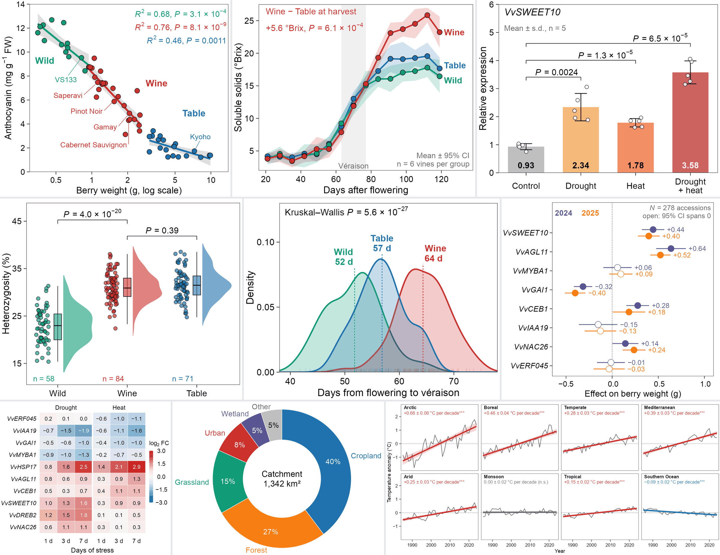
由九张示例图拼成,都用模拟数据在本仓库重画。
Collage of the nine examples, redrawn here from simulated data.
示例 / Examples
点卡片打开画廊大图(含代码与数据);卡片下方的 GitHub 链接打开该图的文件夹。
Click a card to open it in the gallery; the GitHub link below it opens the figure folder.
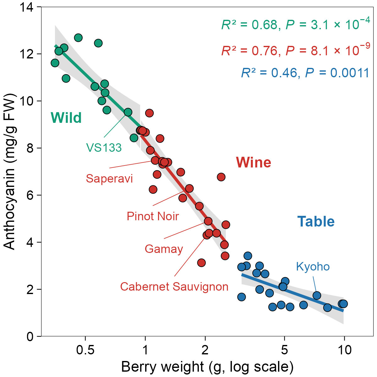 分组散点与回归(house 风格)Scatter with group fits (house style)
correlation/house-scatter · GitHub
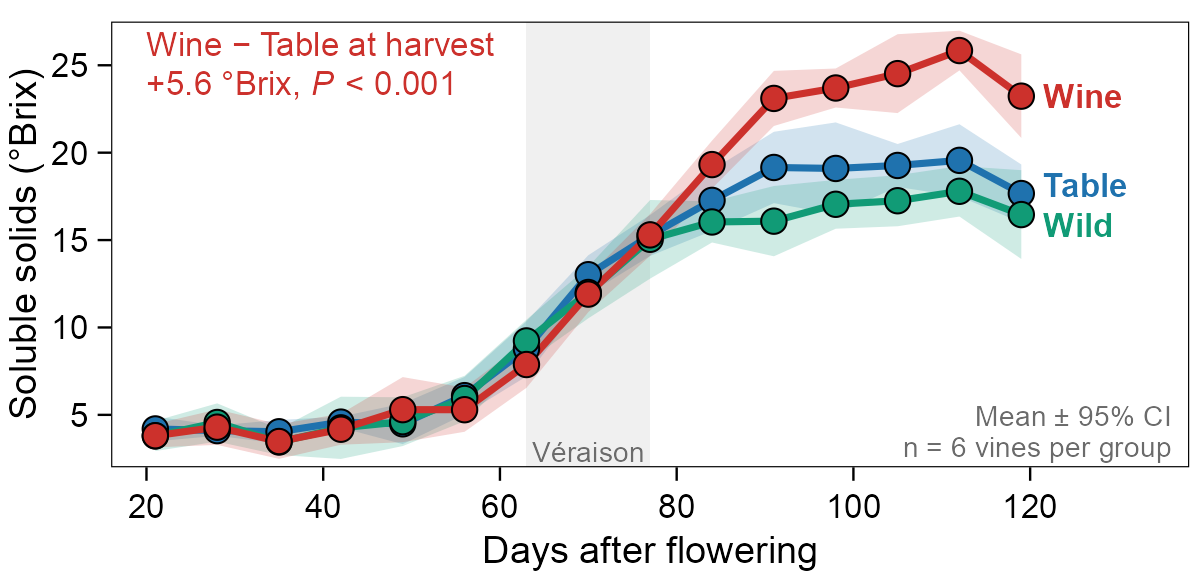 带置信带的折线图(house 风格)Line chart with CI ribbons (house style)
correlation/house-line · GitHub
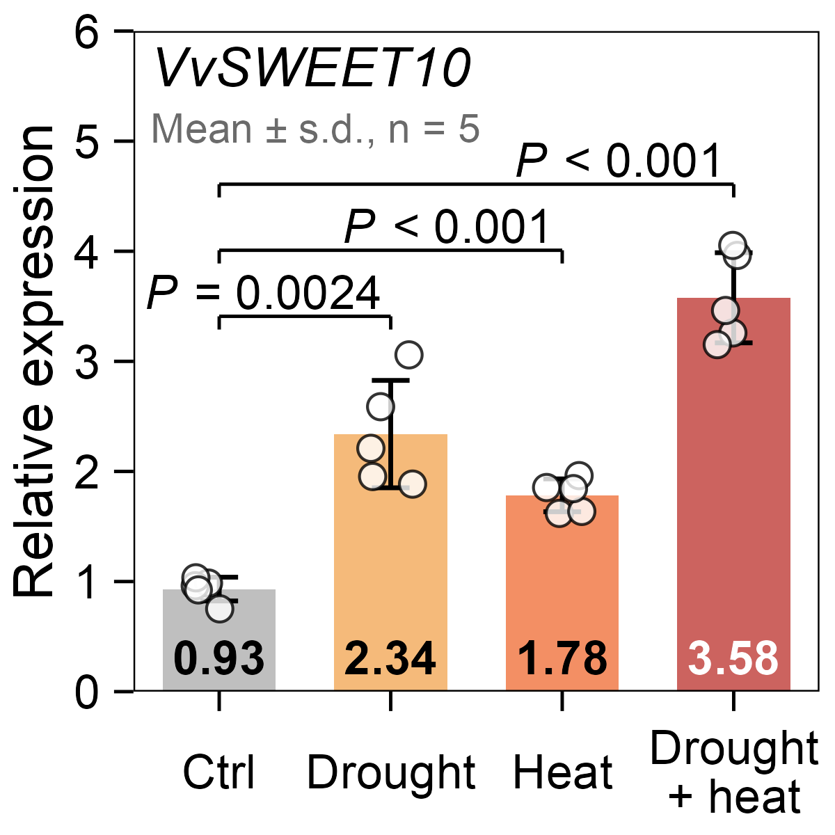 带原始点与 P 值的柱图(house 风格)Bar chart with points and P values (house style)
comparison/house-bar · GitHub
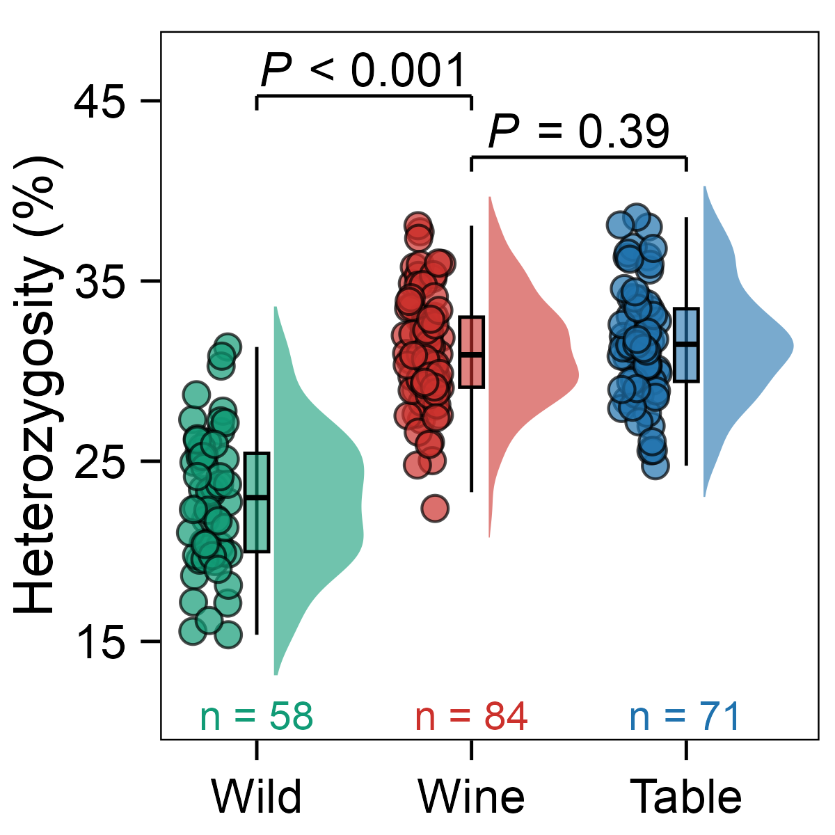 雨云图(house 风格)Raincloud plot (house style)
distribution/house-raincloud · GitHub
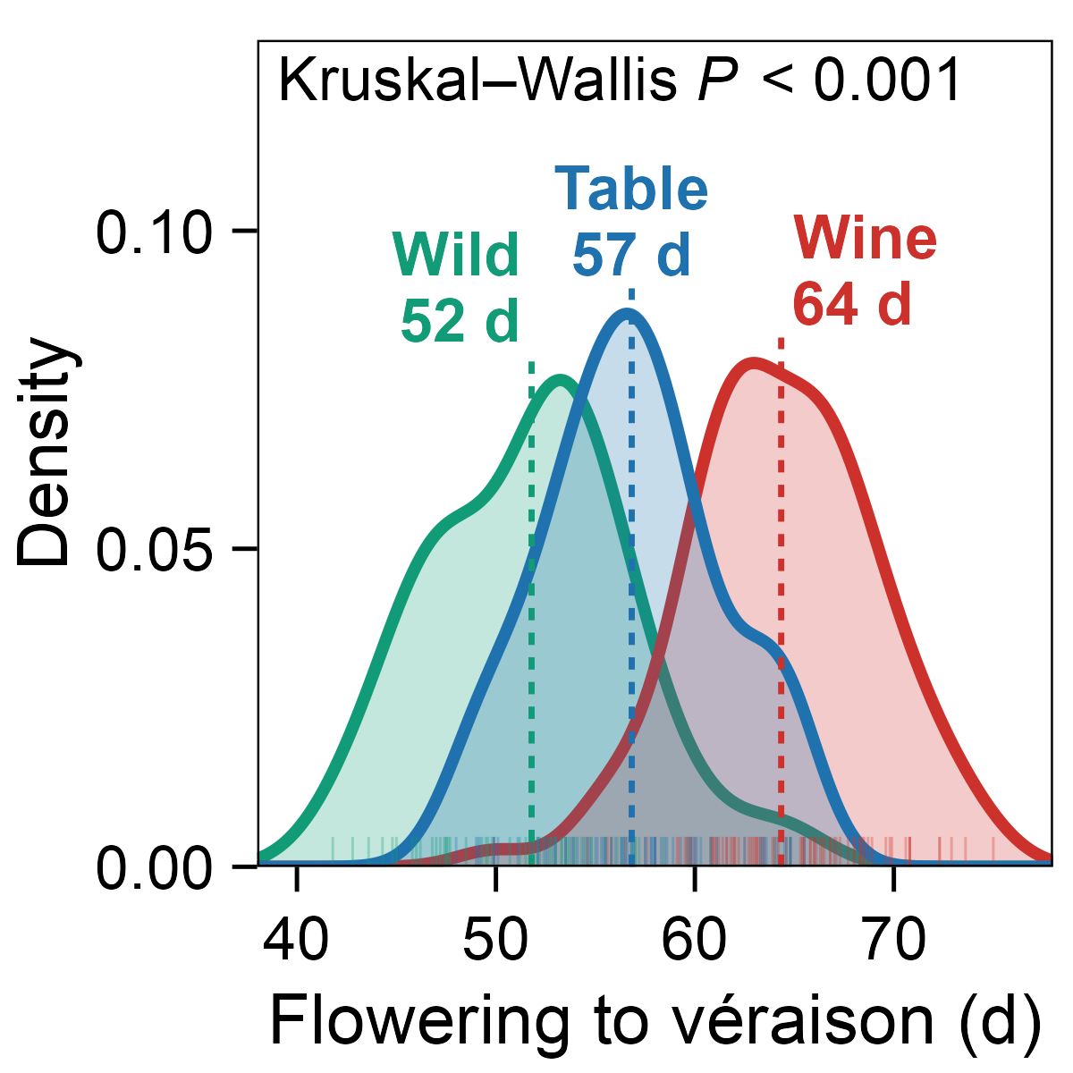 分组密度曲线与均值(house 风格)Density curves with group means (house style)
distribution/house-density · GitHub
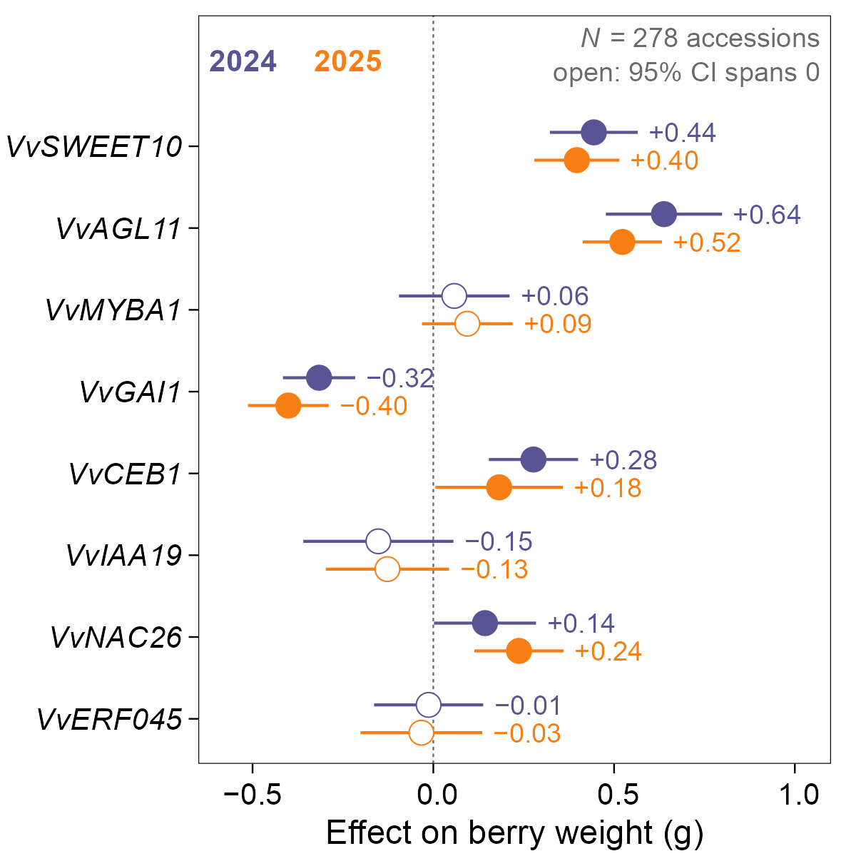 效应量森林图(house 风格)Forest plot of effects (house style)
comparison/house-forest · GitHub
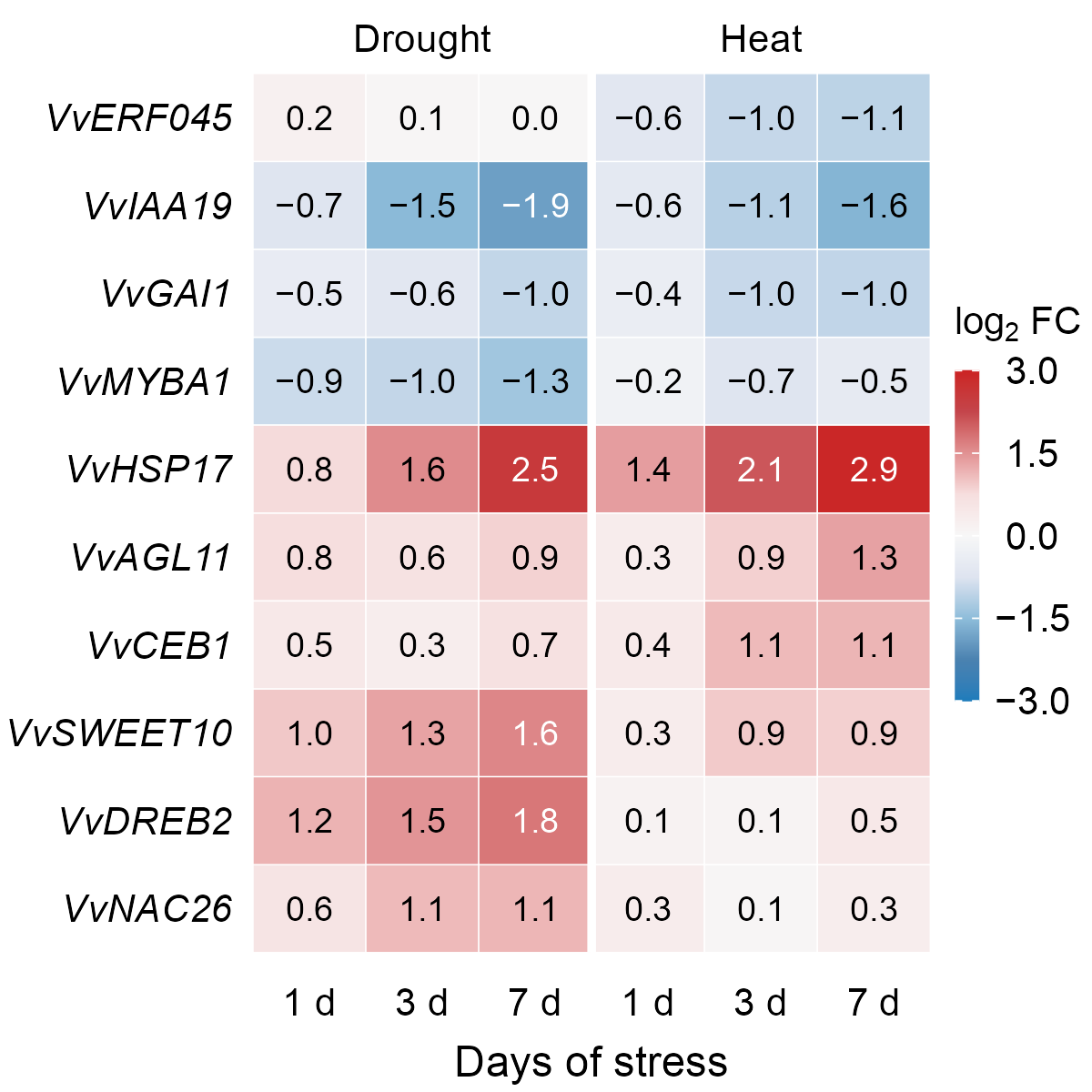 带数值的发散色热图(house 风格)Annotated diverging heatmap (house style)
heatmap/house-heatmap · GitHub
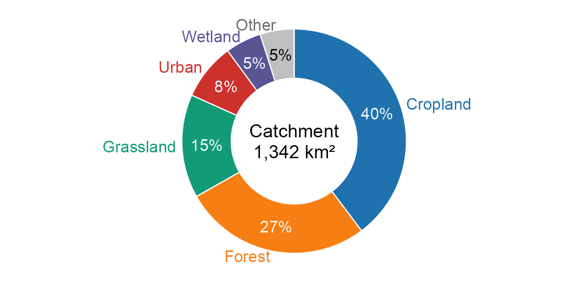 直标环图(house 风格)Donut chart with direct labels (house style)
composition/house-donut · GitHub
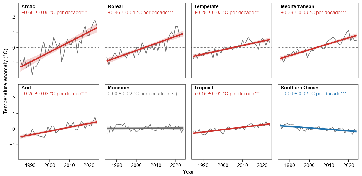 小多图与面板内趋势(house 风格)Small multiples with in-panel trends (house style)
layout/house-small-multiples · GitHub
用法 / Usage
source("../../../styles/r/theme_house.R")theme_house()+pv_palette("house")pv_save_house(p, "figure", cells = "2x1")
中文:theme_house.R 会顺带加载 theme_viz.R。theme_house() 默认 7/8 pt;非用图例不可时用 theme_house(legend = "inside"),放框内右上。尺寸只用网格格数 cells = c(宽, 高)(或 "2x1" 这样的字符串),不在网格上的尺寸直接报错,旧写法 width = "single", height_mm = 76 现在会报错。只有单个面板存成 2×2(89 × 89 mm)时 pv_save_house() 自动 +2 pt(9/10 pt),bump = 0 关掉。多张图拼成一页用 pv_house_mosaic(),见下方第二段代码,导出时 cells 与拼页相同。pv_save_house() 会在输出目录写 <file>.pdf、<file>.png 和 preview.png,覆盖同目录里同名的 preview.png;试跑请在临时目录里进行。
English: theme_house.R also loads theme_viz.R. theme_house() defaults to 7/8 pt; when a legend is unavoidable, use theme_house(legend = "inside") to place it top-right inside the frame. Sizes are given only as grid cells, cells = c(width, height) (or a string such as "2x1"); sizes off the grid are errors, so the old width = "single", height_mm = 76 now fails. pv_save_house() adds +2 pt (9/10 pt) only to a single panel saved at 2×2 (89 × 89 mm); bump = 0 switches this off. To put several plots on one page, use pv_house_mosaic() (second code block below) and export with the same cells. pv_save_house() writes <file>.pdf, <file>.png and preview.png to the output folder and overwrites any preview.png already there, so try it in a scratch folder.
# R: figures/<category>/<slug>/plot.R
source("../../../styles/r/theme_house.R")
library(ggplot2)
df <- data.frame(x = rep(1:10, 3),
                 y = c(1:10, 0.8 * (1:10) + 1, 0.5 * (1:10) + 2),
                 group = rep(c("a", "b", "c"), each = 10))   # or utils::read.csv("data.csv")
p <- ggplot(df, aes(x, y, colour = group)) +
  geom_line(linewidth = pv_house_lw("main")) +
  scale_colour_manual(values = unname(pv_palette("house", 3))) +
  theme_house()
pv_save_house(p, "figure", cells = "2x1")   # 89 x 43 mm

# Python
import sys
from pathlib import Path
import numpy as np
sys.path.insert(0, str(Path(__file__).resolve().parents[3] / "styles" / "python"))
import house
house.apply_house_style()
x = np.arange(1, 11)
fig, ax = house.house_figure(cells="2x1")
ax.plot(x, 0.8 * x + 1, color=house.pv_palette("house")[0])
house.save_house(fig, "figure")
# R: several plots on one page (1 + 1 + 2 cells, 183 x 43 mm)
source("../../../styles/r/theme_house.R")
library(ggplot2)
set.seed(1)
df <- data.frame(x = 1:30, y = 1:30 + rnorm(30, 0, 4))
fit <- summary(lm(y ~ x, data = df))
p_lab <- pv_fmt_p(coef(fit)[2, 4]) # "P < 0.001" at 7/8 pt
p_exact <- pv_fmt_p(coef(fit)[2, 4], exact = TRUE) # "P = m × 10^−k", only for text ≥ 8.6 pt
pa <- ggplot(df, aes(x, y)) +
geom_point(shape = HOUSE_POINT$shape, size = HOUSE_POINT$size, stroke = HOUSE_POINT$stroke,
fill = pv_palette("house")[["blue"]]) +
annotate("text", x = 1, y = 35, hjust = 0, vjust = 1, size = pv_pt2size(7),
label = p_lab, parse = TRUE) +
labs(x = "Dose (mg)", y = "Response", tag = "a") + theme_house()
pb <- ggplot(df, aes(y)) +
geom_histogram(bins = 8, fill = pv_palette("house")[["sky"]], colour = "white") +
labs(x = "Response", y = "Count", tag = "b") + theme_house()
pc <- ggplot(df, aes(x, y)) +
geom_line(linewidth = pv_house_lw("main"), colour = pv_palette("house")[["red"]]) +
labs(x = "Day", y = "Response", tag = "c") + theme_house()
page <- pv_house_mosaic(list(
list(plot = pa, at = c(1, 1), cells = c(1, 1)),
list(plot = pb, at = c(2, 1), cells = c(1, 1)),
list(plot = pc, at = c(3, 1), cells = c(2, 1))
), cells = c(4, 1))
pv_save_house(page, "figure", cells = c(4, 1))
字号层级 / Type scale
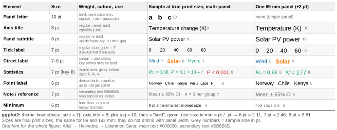
规范摘要(中文)
新加的图一律用 house style;已有的图不重渲染,继续用旧版 theme_viz()。完整规则以 styles/style-contract.md 为准。
| 字号(印刷尺寸) | 默认:刻度 7 pt、轴标题 8 pt(7/8 pt);面板字母 10 pt 粗体小写 a b c;任何文字 ≥6 pt。 只有单个面板存成 2×2(89 × 89 mm)时全部 +2 pt:刻度 9 pt、轴标题 10 pt(9/10 pt), pv_save_house() 自动加;组合图、分面图、拼页不加。字号不随面板缩小。 |
|---|---|
| 网格 | 格宽 43 mm、格间距 3 mm;n 格跨度 = n × 43 + (n − 1) × 3,1–4 格为 43 / 89 / 135 / 181 mm。占满 4 格的边两侧各加 1 mm,导出 183 mm;1–3 格不加边距。宽、高分别算。 |
| 画布与排法 | pv_save_house(p, "figure", cells = c(w, h)),w、h 为 1–4 格。双栏每行 4 格,可排 1+1+1+1 / 1+1+2 / 2+2 / 1+3 / 4;单栏每行 2 格。不在网格上的尺寸报错。多图拼一页用 pv_house_mosaic()。 |
| 轴标题 | 常规字重,不加粗;写变量名和单位,单位用括号,如「温度 (°C)」。 |
| 边框与刻度 | 四边 0.5 pt 黑框,刻度 0.5 pt、长 1 mm、向外;无网格,无次刻度(对数轴除外)。 |
| 线、点与置信带 | 主数据线 1.5 pt,强调 / 拟合线 2.0 pt,次要系列 0.8 pt,参考虚线 0.5 pt,误差棒 0.7 pt。点 shape 21 加黑描边(size = 2.3, stroke = 0.3)。置信带与线同色,透明度 0.2。 |
| 图例与统计量 | 默认不画图例,系列名直接写在图里,文字颜色 = 数据颜色;非用图例不可时放框内右上、无边框。统计量(R²、P、N)写在图内,与组同色。 |
| 字体 | Arial → Helvetica → Liberation Sans → DejaVu Sans;中文思源黑体 / Noto Sans CJK SC。全图一种字体。 |
| 导出 | Cairo PDF(文字保留为文本)+ 600 dpi PNG + 1200 px 宽 preview.png。 |
默认格数
拿不准时用下表;太挤或太空可在网格内升降一档。
| 图型 | 默认 cells |
|---|---|
| 散点 | 1×1 |
| 直方图 / 密度 | 1×1 |
| 箱线 / 小提琴 / 雨云 | 1×1;组多时 2×1 |
| 柱图 | 1×1;类别多时 2×1 |
| 折线 / 时间序列 | 2×1 |
| 堆叠构成 | 2×1 |
| 森林图 | 1×2;行多时 2×2 |
| 热图 | 2×2 |
| 小多图 | 每张小图 1×1 |
| 基因组轨道 / 曼哈顿图 | 4×1 |
Style summary (English)
New figures use the house style. Existing figures are not re-rendered and keep the legacy theme_viz(). The full rules are in styles/style-contract.md.
| Text (print size) | Default: 7 pt ticks, 8 pt axis titles (7/8 pt); 10 pt bold lowercase panel letters; nothing under 6 pt. Only a single panel saved at 2×2 (89 × 89 mm) gets +2 pt on everything: 9 pt ticks and 10 pt axis titles (9/10 pt); pv_save_house() adds it. Compositions, faceted plots and mosaics do not. Text does not shrink with the panel. |
|---|---|
| Grid | Cells 43 mm wide with 3 mm gaps; n cells span n × 43 + (n − 1) × 3, so 1–4 cells are 43 / 89 / 135 / 181 mm. A side spanning all 4 cells gets 1 mm on each end and exports at 183 mm; 1–3 cells get no margin. Width and height are handled separately. |
| Canvas and layout | pv_save_house(p, "figure", cells = c(w, h)), 1–4 cells each way. A double column has 4 cells per row, combined as 1+1+1+1, 1+1+2, 2+2, 1+3 or 4; a single column has 2. Sizes off the grid are errors. Use pv_house_mosaic() to put several plots on one page. |
| Axis titles | Plain weight, not bold; variable name, then the unit in parentheses, e.g. Temperature (°C). |
| Frame and ticks | Four-sided 0.5 pt black frame; ticks 0.5 pt, 1 mm, outward; no grid, no minor ticks (except log axes). |
| Lines, points, CI ribbons | Main lines 1.5 pt, emphasis / fit 2.0 pt, minor series 0.8 pt, dashed reference 0.5 pt, error bars 0.7 pt. Points: shape 21 with a black outline (size = 2.3, stroke = 0.3). CI ribbons in the line colour, alpha 0.2. |
| Legends and statistics | No legend by default: label series in the panel in the series colour. When one is unavoidable, place it top-right inside the frame, with no box. Statistics (R², P, N) go inside the panel in the group colour. |
| Font | Arial → Helvetica → Liberation Sans → DejaVu Sans; Chinese: Source Han Sans / Noto Sans CJK SC. One font per figure. |
| Export | Cairo PDF (text stays text) + 600 dpi PNG + 1200 px wide preview.png. |
Default cells
Use these when unsure; if a figure is crowded or empty, move one size up or down within the grid.
| Chart | Default cells |
|---|---|
| Scatter | 1×1 |
| Histogram / density | 1×1 |
| Box / violin / raincloud | 1×1; 2×1 with many groups |
| Bar | 1×1; 2×1 with many categories |
| Line / time series | 2×1 |
| Stacked composition | 2×1 |
| Forest | 1×2; 2×2 with many rows |
| Heatmap | 2×2 |
| Small multiples | 1×1 per small plot |
| Genome track / Manhattan | 4×1 |
网格版面 / Grid layout
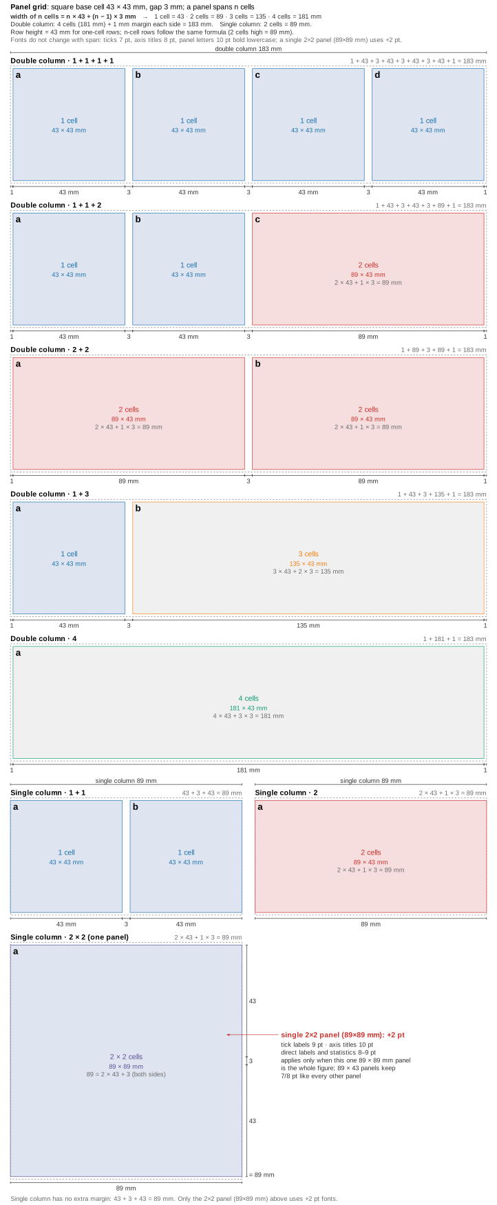
默认尺寸与升档阈值 / Default sizes and when to go up
- 字宽 1.30 mm/字符
- 行高 ≥ 3.5 mm
- 面板内宽 = 格跨度 − 12.7 mm
- 顺序:先缩写或换行,再加宽,最后加高
- Character width: 1.30 mm/char
- Row height: ≥ 3.5 mm
- Inner panel width = cell span − 12.7 mm
- Order: abbreviate or wrap first, then widen, lastly add height
| 图型 Chart | 默认 Default | 组 / 类别 / 集合 > Groups / categories / sets > | 标签字符 > Label chars > | 行 > Rows > | 列 / 交集 > Columns / intersections > | 点 / bins / 面板 > Points / bins / panels > | 升到 Up to |
|---|---|---|---|---|---|---|---|
| Scatter 散点 | 1×1 | 3 | — | — | — | 2,000 | 2×2 |
| Line 折线 | 2×1 | 4 | — | — | — | 12 | 4×1 / 2×2 |
| Bar 柱图 | 1×1 | 4 | 4 | — | — | — | 2×1 |
| Box / violin | 1×1 | 4 | — | — | — | — | 2×1 |
| Raincloud(横向 / horizontal) | 1×1 | 4 | — | — | — | — | 2×2 |
| Forest 森林图 | 1×2 | — | 17 | 21 | — | — | 2×2 |
| Heatmap 热图(印数值 / values) | 2×2 | — | 10 | 21 | 17 | — | 2×3 / 2×4 |
| Histogram / density | 1×1 | 3 | — | — | — | 37 | 2×1 |
| Donut 环图 | 1×1 | 4 | 5 | — | — | — | 2×1 |
| Stacked bar 堆叠条 | 1×1 | 4 | — | — | — | — | 1×2 / 2×1 |
| Small multiples 小多图 | 2×2 | — | — | — | — | 4 | 4×2 / 4×3 |
| UpSet(拼图 / mosaic) | 3×1 | 5 | 10 | — | 15 | — | 4×1 / 3×2 |
| Manhattan / genome track | 4×1 | 19 | — | — | — | — | 4×1 + 2×1 |
| 示例 / Examples | |||||||
house-mosaic-transcriptome | 4×3 | 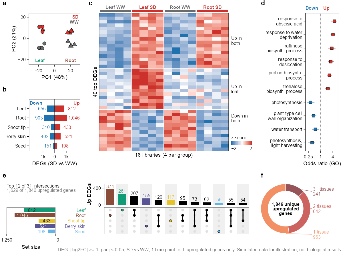 | |||||
house-mosaic-aba-kinetics | 2×4 | 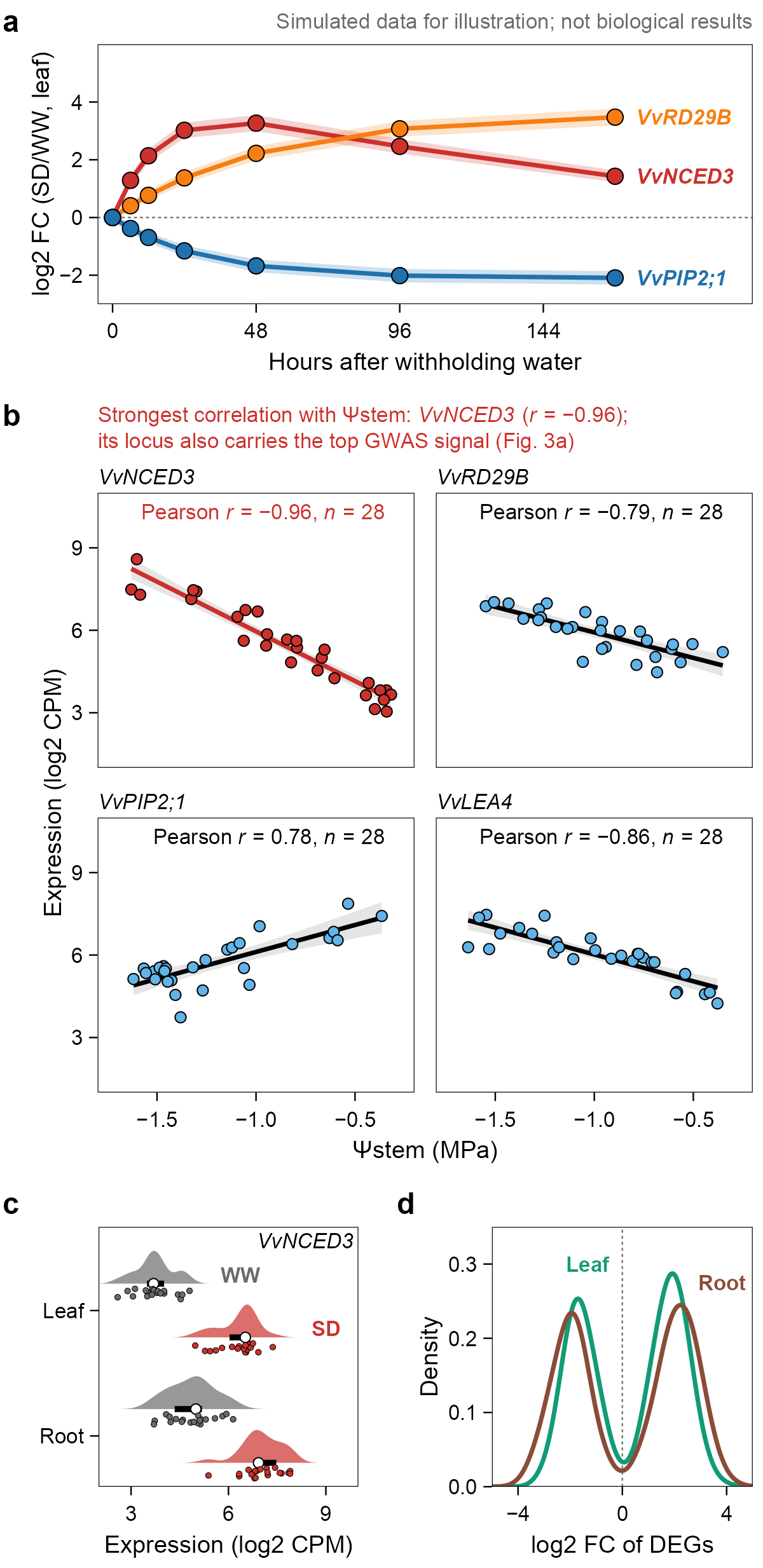 | |||||
house-mosaic-gwas | 4×2 | 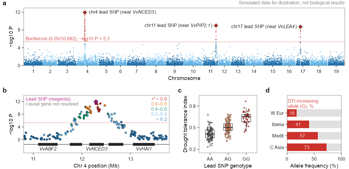 | |||||
参考示例 / Examples: house-mosaic-transcriptome (4×3) · house-mosaic-aba-kinetics (2×4) · house-mosaic-gwas (4×2). 测量方法与每档容量 / Method and capacity per size: styles/style-contract.md.
示意图与架构图 / Schematics
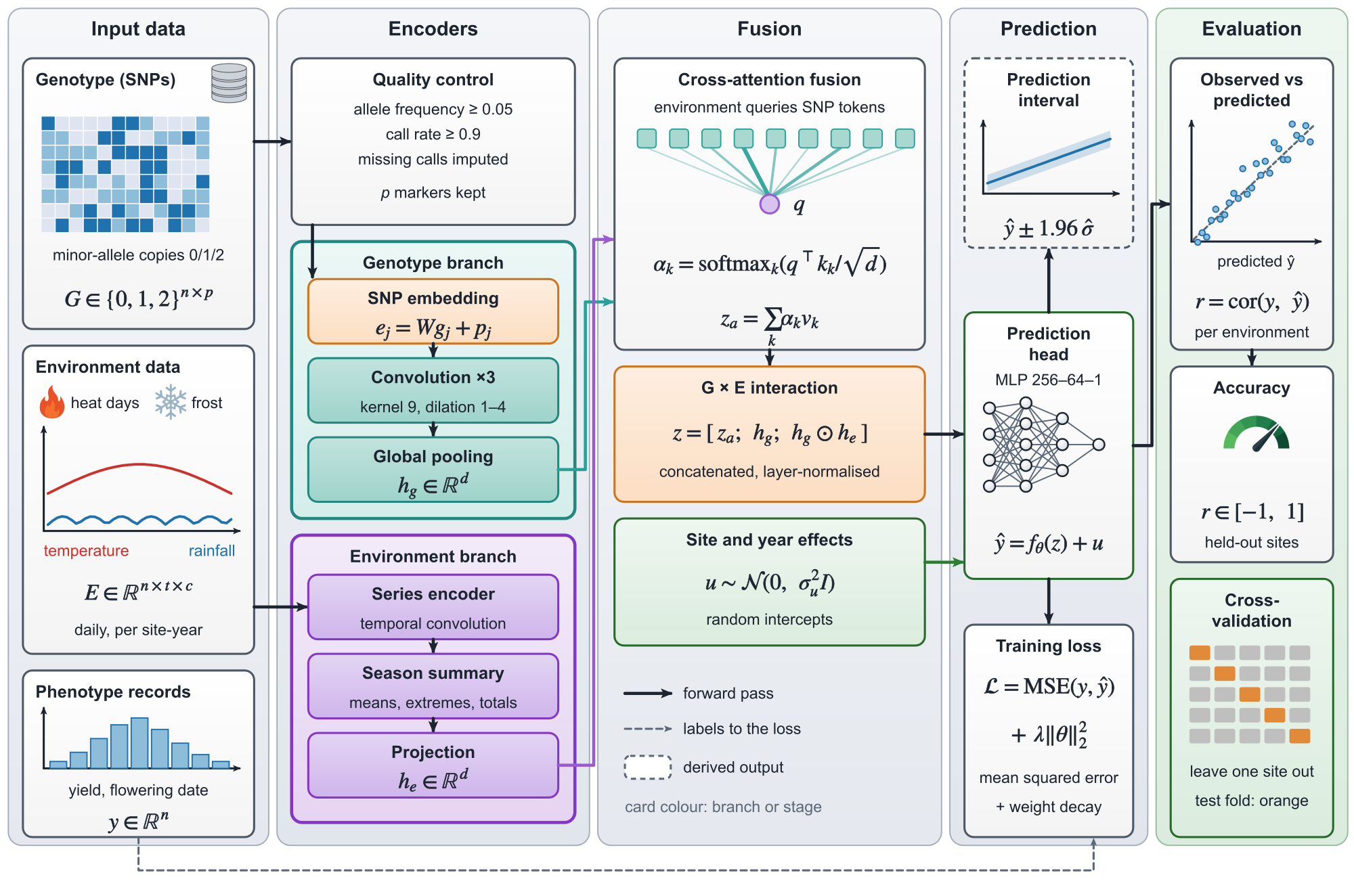
浏览全套可下载图示 / View downloadable schematics
中文:新示意图(模型架构、流程、方法框图)用 Python 脚本生成可编辑 SVG,取代 draw.io;旧 draw.io 图保留不动。
- Python 脚本生成可编辑 SVG
- 线宽和字号按参考图实测
- 公式转成矢量路径
- 嵌入 AI 生成图标,保留矢量备用图标
- 对照参考图至少迭代 3 轮
数值、检查和交付要求以 styles/style-contract.md 为准;示例脚本见 docs/house-style/arch/。
English: New schematics (model architectures, workflows, method diagrams) are editable SVG generated by a Python script, replacing draw.io; existing draw.io figures stay as they are.
- Generate an editable SVG with a Python script
- Measure stroke widths and font sizes on the reference
- Convert formulas to vector paths
- Embed AI-generated icons and keep vector fallback icons
- Iterate against the reference at least three times
Numbers, checks and deliverables are defined in styles/style-contract.md; the example script is in docs/house-style/arch/.
色板 / Palettes
| 名字 / Name | 中文用途 | Use | 色值 / Colours |
|---|---|---|---|
house | 分类,按序取,≤6 个彩色系列,其余用灰 | Categories, in order, ≤6 coloured series, the rest grey | #1F72AE#F77E12#119B76#CC312C#595594#62B4E7#E6C32A#A8127F#8A4C38 |
house_div | 蓝–红发散,0 居中 | Blue–red diverging, centred on 0 | #1D7CBB#4A82B0#8EBDDA#DEE4F0#F7F7F7#F6DEDE#E19193#C4454B#CB2223 |
ssp | 情景 | Scenarios | Historical #000000SSP1-2.6 #3A9CFESSP2-4.5 #F79423SSP3-7.0 #FD3B3BSSP5-8.5 #9C2125 |
house_warm | 暖色顺序 | Warm sequential | #FBD6A0#F5BA7A#F38F64#CC635F#965459 |
house_grey | 文字、参考线、置信带 | Text, reference lines, CI ribbons | #000000#333333#6B6B6B#757575#BFBFBF#E0E0E0#F0F0F0 |
geo | 地理群体渐变(6色按西至东取) | Geographic population gradient (6 colors west to east) | #c5c838#eaa944#e17d52#b93234#3e9349#2c69a6 |
chrom12 | 染色体交替色(12色浅深交错) | Chromosome alternating colors (12 colors alternating light and dark) | #a3c7da#2072aa#accc8a#339a39#e49698#d02623#ecba73#e17927#c4b1d1#623f88#efe89c#ab5a29 |
中文说明
- geo 提供 6 种颜色,适用于地理或群体渐变(PCA 着色按地理顺序)。
- 当 n > 6 时,pv_palette("geo", n) 会自动插值。
- chrom12 提供 12 种交替色,相邻染色体一浅一深,适用于曼哈顿图或基因组轨道。
- 若染色体数量超过 12 条,系统会报错。
- 标签对比规则:组色对白底对比度 ≥ 3:1 时标签用组色,否则用 #1A1A1A。
English Description
- The geo palette offers 6 colors for geographic or population gradients. PCA coloring follows geographic order.
- The function pv_palette("geo", n) interpolates colors when n > 6.
- The chrom12 palette offers 12 alternating light and dark colors for Manhattan plots and genome tracks.
- Requesting more than 12 colors will result in an error.
- Label contrast rule: Use group color for labels if contrast against white background is ≥ 3:1, otherwise use #1A1A1A.
# R
cols <- pv_palette("geo")              # 6 colours; pv_palette("geo", 9) ramps
chr_cols <- pv_palette("chrom12")      # 12 colours; n > 12 is an error
# Python
cols = house.pv_palette("geo")
chr_cols = house.pv_palette("chrom12")
参考 / References
只列链接与图号;参考图不进仓库。
Links and figure numbers only; no reference images are stored here.
26 条参考 / 26 references
| 来源 / Source | 图号 / Figure |
|---|---|
| One Earth 2024 | Fig. 1 |
| Sci. Adv. 2023 | Fig. 3 |
| Nat. Energy 2024 | Fig. 1 |
| Joule 2024 | Fig. 3 |
| Joule 2025 | Fig. 6 |
| PNAS 2026 | Fig. 2 |
| Nat. Clim. Change 2024 | Fig. 3 |
| Sci. Adv. 2025 | Fig. 3 |
| Nat. Sustain. 2025 | Fig. 3 |
| PNAS 2024 | Fig. 3 |
| One Earth 2025 | Fig. 2 |
| Nat. Energy 2026 | Fig. 3 |
| Nat. Commun. 2023 | Fig. 2 |
| Nat. Commun. 2025 | Fig. 5 |
| Nat. Commun. 2026 | Fig. 6 |
| Nat. Commun. 2026 | Fig. 5 |
| Nat. Commun. 2026 | Fig. 5 |
| Nat. Commun. 2024 | Fig. 5c |
| Nat. Commun. 2024 | Fig. 1a |
| Nat. Commun. 2025 | Fig. 1a, Fig. 5a |
| One Earth 2023 | Fig. 1B |
| Nat. Commun. 2024 | Fig. 4c |
| One Earth 2023 | Fig. 1 |
| Bizard | gallery page |
| Bizard | gallery page |
| R Graph Gallery | gallery page |